Quickstart

ATHENA is an open-source computational framework written in Python that facilitates the visualization, processing and analysis of (spatial) heterogeneity from spatial omics data. ATHENA supports any spatially resolved dataset that contains spatial transcriptomic or proteomic measurements, including Imaging Mass Cytometry (IMC), Multiplexed Ion Beam Imaging (MIBI), multiplexed Immunohistochemisty (mIHC) or Immunofluorescence (mIF), seqFISH, MERFISH, Visium.

Important

You are strongly advised to read the sections:

• Note on Phenotype Encodings

• Note on Segmentation Masks

at the end of this document.

Requirements

To use all the capabilities of ATHENA one needs the (cell-) segmenation masks for a sample and the omics-profiles of the observations in the sample (as extracted from the high-dimensional images produced by different omics-technologies).

However, it is also possible to use ATHENA (with some limitations) without segmentation masks and the omics-profiles and just the single-observation coordinates and a classification of those observations (phenotypes).

Further Resources

• A more comprehensive tutorial on IMC data can be found here

• A tutorial on how to load your data can be found here

import athena as ath
import numpy as np
import pandas as pd
import seaborn as sns
from pathlib import Path

pd.set_option("display.max_columns", 5)
print(ath.__version__)

<frozen importlib._bootstrap>:219: RuntimeWarning: numpy.ndarray size changed, may indicate binary incompatibility. Expected 80 from C header, got 88 from PyObject


0.1.2

Load Example Data

To use ATHENA you need to load the data in a SpatialOmics instance (see below, here for a general description and here for a more detailed tutorial). The structure of the SpatialOmics instance is very similar to the AnnData.

For this tutorial we provide a small example of a populated SpatialOmics instance. Meta data for each stored sample can be found in so.spl. You can access the data by indexing the different attributes by the sample name (so.X[spl], so.obs[spl, …).

so = ath.dataset.imc_quickstart()
so

INFO:numexpr.utils:NumExpr defaulting to 8 threads.


warning: to get the latest version of this dataset use `so = sh.dataset.imc(force_download=True)`






SpatialOmics object with 5505 observations across 2 samples.
    X: 2 samples,
    spl: 2 samples,
        columns: ['pid', 'cell_count', 'immune_cell_count']
    obs: 2 samples,
        columns: ['meta_label', 'id', 'core', 'cell_type', 'meta_id', 'CellId', 'x', 'cell_type_id', 'tumor_immune_id', 'tumor_immune', 'phenograph_cluster', 'y']
    var: 2 samples,
        columns: ['target', 'fullstack_index', 'metal_tag', 'feature_type', 'channel', 'full_target_name']
    G: 0 samples,
        keys: []
    masks: 2 samples
        keys: [{'cellmasks'}]
    images: 0 samples

samples = so.spl.index
samples

Index(['SP43_75_X2Y5', 'SP41_239_X11Y3_165'], dtype='object', name='core')

How to Create a SpatialOmics Instance with Dummy Data

# create dummy data

n_obs = 100  # number of observations (cells)
n_var = 5  # number of features
samples = ['sample_'+ str(i) for i in range(5)]  # sample names
mask_dim = [100,100]  # dimension of segmentation masks

# sample-level meta data
spl = pd.DataFrame({'samples': samples, 'age': np.random.choice(range(50,80), len(samples))}).set_index('samples')

# observation-level meta data
obs = pd.DataFrame({
    'phenotype': range(n_obs),
    'x': np.random.randint(0, mask_dim[0], n_obs),
    'y': np.random.randint(0, mask_dim[1], n_obs)})

# observation-level omics profiles
X = pd.DataFrame(np.random.rand(n_obs, n_var), columns=['var_' + str(i) for i in range(n_var)])
# high-dimensional images of samples, first dimension is the number of features, i.e. multiplexing
img = np.random.rand(n_var, *mask_dim)
# segmentation masks of images
mask = np.zeros(mask_dim, dtype=int)
# feature annotation
var = pd.DataFrame({'target': ['var_' + str(i) for i in range(n_var)]})

# create SpatialOmics instance

from spatialOmics import SpatialOmics
dummy = SpatialOmics()

dummy.spl = spl
for spl in samples:
    dummy.obs[spl] = obs
    dummy.X[spl] = X
    dummy.var[spl] = var
    dummy.images[spl] = img
    dummy.masks[spl] = {'cellmasks': mask}
    
dummy

SpatialOmics object with 500 observations across 5 samples.
    X: 5 samples,
    spl: 5 samples,
        columns: ['age']
    obs: 5 samples,
        columns: ['y', 'phenotype', 'x']
    var: 5 samples,
        columns: ['target']
    G: 0 samples,
        keys: []
    masks: 5 samples
        keys: [{'cellmasks'}]
    images: 5 samples

Minimal Working Example

Depending on your use case you do not need to populate all attributes of the SpatialOmics instance.

For a minimal working example you only need to populate the .obs attribute with the observation coordinates and a label.

dummy_min = SpatialOmics()
dummy_min.obs[spl] = obs
dummy_min

SpatialOmics object with 100 observations across 1 samples.
    X: 0 samples,
    spl: 0 samples,
        columns: []
    obs: 0 samples,
        columns: ['y', 'phenotype', 'x']
    var: 0 samples,
        columns: []
    G: 0 samples,
        keys: []
    masks: 0 samples
        keys: [set()]
    images: 0 samples

Sample-level Meta Data

Sample-level meta data is stored in the so.spl attribute but not required to use ATHENA.

so.spl.head(3) 

	pid	cell_count	immune_cell_count
core
SP43_75_X2Y5	75	2771	940
SP41_239_X11Y3_165	239	2734	412

Observation-level Meta Data

Observation-level meta data is stored in the so.obs attribute and required to use ATHENA. At least the coordinates of the observations along with some classification of those (phenotypes) are required.

spl = so.spl.index[0]
so.obs[spl].head()

	core	meta_id	...	y	x
cell_id
1	SP43_75_X2Y5	9	...	1.142857	33.107143
2	SP43_75_X2Y5	3	...	4.868613	43.693431
3	SP43_75_X2Y5	10	...	5.467391	61.326087
4	SP43_75_X2Y5	8	...	2.353659	79.987805
5	SP43_75_X2Y5	3	...	2.026316	128.302632

5 rows × 12 columns

Observation-level Omics Profiles

The omics-profiles of the obserations are stores in the so.X attribute. These are the gene / protein expression values of the observations (most likely single cells or patches). You only need to provide this information if you want to use metrics.quadratic_entropy().

so.X[spl].head()

target	H3	H3K28me3	...	PARP	DNA2
cell_id
1	8.252318	0.442500	...	0.674024	9.002035
2	12.754854	1.436547	...	0.852686	19.567230
3	1.946717	0.470739	...	0.858645	2.316239
4	7.552009	0.562183	...	0.939330	8.991525
5	15.079700	0.492224	...	0.828238	12.647001

5 rows × 34 columns

Compute Graphs

ATHENA can construct knn, radius and contact graphs. By default, ATHENA tries to build the graphs from segmentation masks. Without segmentation masks, one can only use the kNN and radius graph functionality of ATHENA. For the contact graph the segmentation masks are required. See the main tutorial to see how the graph construction can be customized.

From Segmentation Masks

Provide the spatialOmics instance and sample name for which the graph should be computed. Furthermore, builder_type defines the type of graph that is constructed and mask_key the segmentation masks that should be used (stored at so.masks[spl][MASK_KEY])

ath.graph.build_graph(so, spl, builder_type='knn', mask_key='cellmasks')
so.G[spl].keys()  # graphs are stored at so.G[spl]

dict_keys(['knn'])

One can build multiple graph-representations for each sample by simply calling build_graph again with another builder_type

ath.graph.build_graph(so, spl, builder_type='radius', mask_key='cellmasks')
so.G[spl].keys()  # graphs are stored at so.G[spl]

dict_keys(['knn', 'radius'])

From Coordinates

One can build the knn and radius graphs from coordinates only by setting mask_key=None and providing the column names of the coordinates with coordinate_keys.

ath.graph.build_graph(so, spl, builder_type='knn', mask_key=None, coordinate_keys=('x', 'y'))
ath.graph.build_graph(so, spl, builder_type='radius', mask_key=None, coordinate_keys=('x', 'y'))
so.G[spl].keys()  # graphs are stored at so.G[spl]

dict_keys(['knn', 'radius'])

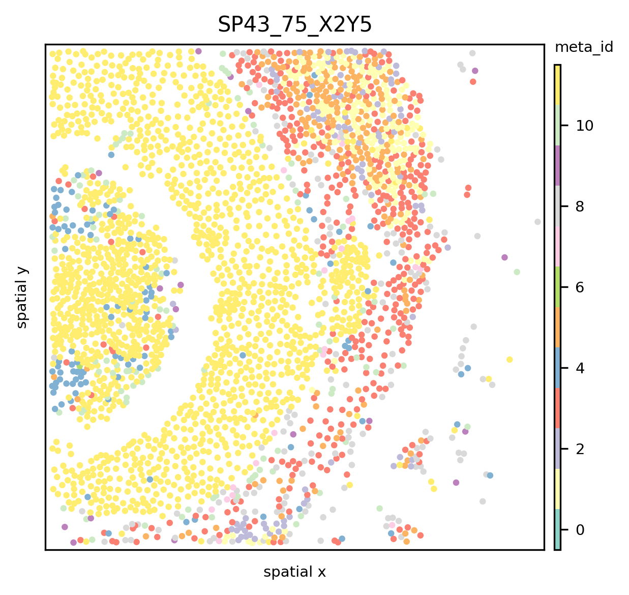
Visualise the Data

For some of the plotting functionalities ATHENA requires the x,y coordinates of each observation. They can be extracted from segmentation masks with

ath.pp.extract_centroids(so, spl, mask_key='cellmasks')

The data can then be visualised with

ath.pl.spatial(so, spl, attr='meta_id')

/Users/art/Documents/projects/athena/athena/plotting/visualization.py:217: UserWarning: Matplotlib is currently using module://matplotlib_inline.backend_inline, which is a non-GUI backend, so cannot show the figure.
  fig.show()

or if one wants to use custom coordinates, one can provide coordinate keys that are stored in the so.obs[spl] dataframe ATHENA should use

ath.pl.spatial(so, spl, attr='meta_id', coordinate_keys=['x', 'y'])

See the main tutorial and the docs to see how the plotting can be customized.

Compute Metrics

Once the graphs are built we can use the quantifications methods from the ath.metrics and the ath.neigh module. Again, provide the spatialOmics instance and the sample name for which the metric should be computed. Furthermore, since ATHENA quantifies the phenotypic heterogeneity in the data, provide the column name that indicates the different phenotypes of each observation with attr and specify the graph topologie to use with graph_key.

Most of the metrics can be computed either on a sample-level (i.e. 1 value per sample) or on a observation-level (i.e. 1 value per observation). This behaviour can be controlled by setting local={True,False}.

# compute shannon entropy for each observation, once for the radius graph and once for the knn graph
ath.metrics.shannon(so, spl, attr='meta_id',graph_key='radius')
ath.metrics.shannon(so, spl, attr='meta_id',graph_key='knn')

# compute the shannon entropy for the whole sample
ath.metrics.shannon(so, spl, attr='meta_id', local=False)

The results for local=True (default) are stores in so.obs as {method}_{attr}_{graph_key}.

so.obs[spl].head()

	core	meta_id	...	shannon_meta_id_radius	shannon_meta_id_knn
cell_id
1	SP43_75_X2Y5	9	...	1.921928	1.918296
2	SP43_75_X2Y5	3	...	1.918296	1.918296
3	SP43_75_X2Y5	10	...	2.446439	2.521641
4	SP43_75_X2Y5	8	...	2.419382	2.128085
5	SP43_75_X2Y5	3	...	1.870254	1.459148

5 rows × 14 columns

The results for local=False are stored in so.spl

so.spl.loc[spl].head()

pid                    75.000000
cell_count           2771.000000
immune_cell_count     940.000000
shannon_meta_id         3.311329
Name: SP43_75_X2Y5, dtype: float64

Note On Phenotype Encodings

We advise the users to use numeric phenotype encodings when computing metrics. If one has label names stored in a pd.DataFrame as label_names one can easily create numeric labels by

df = pd.DataFrame({'label_names': ['A', 'B', 'B', 'C']})
df['labels_names_id'] = df.groupby('label_names').ngroup()

Furthermore, some functions require a strict categorical encoding. Thus the columns dtype should be set to categorical and include all categories across the samples. This can be achived by running the following snippet for all categorical columns in so.obs[spl]

# collect all occurences in the dataset
i = set()
for spl in so.spl.index:
    i.update(so.obs[spl]['meta_id'].values)

# define categorical dtype
dtype = pd.CategoricalDtype(i)
for spl in so.spl.index:
    so.obs[spl].loc[:,'meta_id'] = so.obs[spl]['meta_id'].astype(dtype)

Note On Segmentation Masks

Segmentation masks should be stored as np.ndarray and have int encodings with 0 being background. The labels do not need to be sequential but aligned with the index in so.obs[spl], i.e. the label of the segmentation mask should be the same as in the index of the so.obs dataframe for a given observation. One can test that the labels overlap

ids = np.unique(so.masks[spl]['cellmasks'])
ids = ids[ids!=0]  # remove background label
s_mask = set(ids)
s_obs = set(so.obs[spl].index.values)
assert len(s_obs - s_mask) == 0
assert len(s_mask - s_obs) == 0